
Lookup

HLOOKUP and VLOOKUP are functions in Microsoft Excel that allow you to use a section of your spreadsheet as a lookup table.
When the VLOOKUP function is called, Excel searches for a lookup value in the leftmost column of a section of your spreadsheet called the table array. The function returns another value in the same row, defined by the column index number.
HLOOKUP is similar to VLOOKUP but searches a row instead of a column, and the result is offset by a row index number. The V in VLOOKUP stands for vertical search (in a single column), while the H in HLOOKUP stands for horizontal search (within a single row).
VLOOKUP example
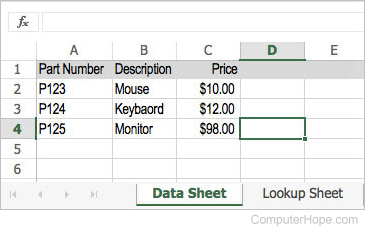
Let's use the workbook below as an example which has two sheets. The first is called "Data Sheet." On this sheet, each row contains information about an inventory item. The first column is a part number, and the third column is a dollar price.
The second sheet is called "Lookup Sheet" and it contains a formula that uses VLOOKUP to look up data on the Data Sheet. In the screenshot below, cell B2 is selected, and its formula is listed in the formula bar at the top.
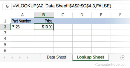
The value of cell B2 is the formula =VLOOKUP(A2,'Data Sheet'!$A$2:$C$4,3,FALSE).
The above formula will populate the B2 cell with the part price identified in cell A2. If the price changes on the Data Sheet, the value of cell B2 on the Lookup Sheet will be updated automatically to match. Similarly, if the part number in cell A2 on the Lookup Sheet changes, cell B2 automatically updates with the price of that part.
Let's look at each element of the example formula in more detail.
| Formula Element | Meaning |
|---|---|
| = | The equals sign (=) indicates that this cell contains a formula, and the result should become the cell's value. |
| VLOOKUP | The name of the function. |
| ( | An opening parenthesis indicates that the preceding name VLOOKUP was the name of a function. It also begins a list of comma-separated arguments to the function. |
| A2 | A2 is the cell containing the value to look up. |
| 'Data Sheet'!$A$2:$C$4 | The second argument is the table array. It defines an area on a sheet to be used as the lookup table. The leftmost column of this area is the column that contains the Lookup Value. The table array argument takes the general form: 'SheetName'!$col1$row1:$col2$row2 The first part of this expression identifies a sheet, and the second part identifies a rectangular area on that sheet. Specifically:
The leftmost column of the table array must contain your lookup value. Always define your table array so the leftmost column contains the value you're looking up. This argument is required. |
| 3 | The third VLOOKUP argument is the Column Index Number. It represents the number of columns offset from the leftmost column of the table array, where the result of the lookup will be found. For instance, if the leftmost column of the lookup array is C, a Column Index Number of 4 would indicate that the result should come from the E column. In our example, the leftmost column of the table array is A, and we want a result from the C column. A is the first column, B is the second, and C is the third, so our column index number is 3. This argument is required. |
| FALSE | The fourth argument is the Range Lookup value. It can be either TRUE or FALSE, specifying whether Excel should perform the lookup using "exact lookup" or "range lookup."
If you're not sure which type of match to use, choose FALSE for an exact match. If you choose TRUE for a range lookup, ensure the data in your table array's leftmost column is sorted in ascending order (least-to-greatest). Otherwise, the results are incorrect. This argument is optional. If you omit this argument, an exact lookup will be performed. |
| ) | A closing parenthesis indicates the end of the argument list and the end of the function. |
Remember the following about lookups
- The lookup value must be in the leftmost column of the table array. If not, the lookup function fails.
- Ensure that every value in the leftmost column of the table array is unique. If you have duplicate values in the column where the lookup takes place, the results of VLOOKUP are not guaranteed to be correct.