
Excel overview
Excel basics
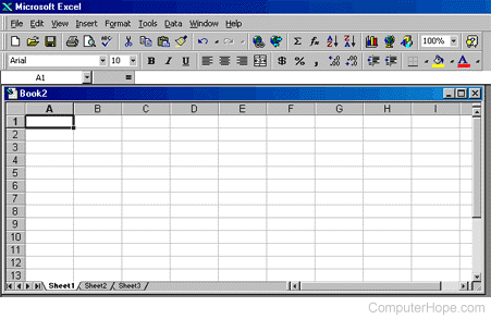
Below is a picture of what Microsoft Excel's main screen may look. As you can see, the working environment is several boxes, called cells. Across the top, there are alphabetic letters, which represent columns. Columns are rows that lay vertically. Along the left side of the screen are numbers, which represent the rows and go horizontally, or left to right.
Formatting cells
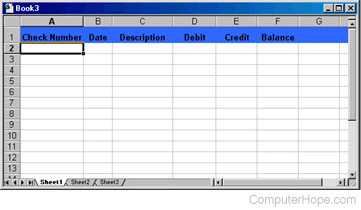
Before creating a spreadsheet, the user must decide how the spreadsheet is going to work and what its function is. We are going to create a layout of a basic checking account spreadsheet to show you some key features of Excel. As you can see with the bottom example, we have created a blue bar to distinguish the categories of the checking account. To change the colors of cells, you first must highlight the cells you want to change colors.
To highlight the whole row or column, click the letter or number of the row or column that you want to highlight.
Once highlighted, click Format, Cells, and then Patterns. Under Pattern, select the color or pattern for the cells.
Formulas
Spreadsheets are used because they calculate values in other cells without you having to do any and be automatically updated if any cell is changed.
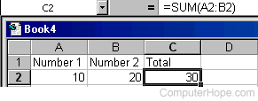
The image above is an example of a simple formula that can be extended or used in your spreadsheets. In the top-right corner of the image is =SUM(A2:B2), an example of an Excel formula. In parentheses is A2:B2, the cells A2 (10) and B2 (20) being added together, represented by a colon between the two cells.
The summed total of 30 is displayed in C2, or whichever cell the formula is entered. So if A2 was to changed to 20, C3 would automatically be updated to 40 because 20 + 20 = 40.
Numbering
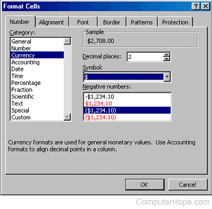
When creating information on the spreadsheets, changing the number format may be required to create a dollar format, such as $5.45 instead of 5.45. Number formats help readers understand the number value. Select the cells you want to change the format of and click Format. In the Format Cells window, on the Number tab as shown below, notice the Category section that lets you choose the scheme for the numbers. With Currency, additional options can be set, such as setting the decimal place, which defaults to 2. The default symbol is $, which can be changed, if desired.
If you did not highlight a cell with a number format, you will not get an example as shown below.
Charts
There are many aspects to point out. First, before attempting to create a chart, it is easier to highlight the values that you want included in the chart.
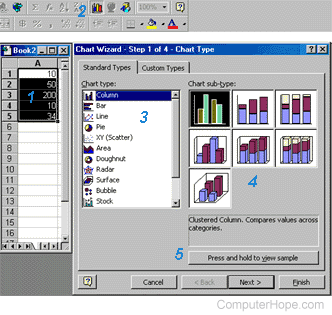
In the picture above, we have a small spreadsheet on the left side, which is represented by #1. The values in this spreadsheet are all highlighted.
Once highlighted, click the Chart Wizard icon at the top of the picture, which is represented by #2.
Once you have clicked the Chart Wizard button, it brings up a wizard that helps you go through creating a chart. Represented by #3, there's a Chart Type section, which lets you select the chart you want to use, such as bar, pie, stock, etc.
After selecting a chart type, choose the chart sub-type (if applicable) you want to create, represented by #4.
Once you have chosen the type of chart you want, before clicking the Next button, click and hold the Press and hold to view sample button, represented by #5. This shows you a preview of what your graph is going to look.
After viewing a sample of your chart, click Next and continue through the wizard for additional features. You can also click Finish to complete the chart.
Freeze
Freeze is an extremely nice feature that lets you work with large spreadsheets, without losing the capability of seeing what each row represents. To create a freeze, first highlight the row under the row(s) that you want to freeze. For example, if you wanted to freeze row number one, you would highlight row number two by clicking number two. Once the row is highlighted, click the drop-down menu at the top of the screen that says window, then click Freeze.
Now, if you were to enter some information in multiple rows of a column and scroll down, notice all rows except row one scrolls down. An example of how you can use this is to enter your checking account information in row one, as shown in the example below. Freeze row number one, then you can have several pages of information that you can scroll down and never lose track of what each column represents.