
How to change the name of the column headers in Excel

In Microsoft Excel, the column headers are named A, B, C, and so on by default. Some users want to change their names to something more meaningful. Unfortunately, Microsoft does not allow the header names to be changed in Excel, but alternative options exist for setting and displaying custom column headers.
The same applies to row names or numbering in Excel, which also may not be changed. Alternatively, add the desired row names in column A for the corresponding rows.
To learn how to create and display meaningful column header names, select from the list below and follow the steps.
We recommend utilizing the first two, if not all three, sections to get the full effect.
Add header names in the first row
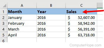
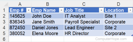
While Excel won't let you change the default column header names, custom header names can be added in the first row.
- Click any cell in the first row of the worksheet and insert a new row above the first row.
- In the inserted row, enter the preferred name for each column.
- To make the row of column names more noticeable, increase the text size, make the text bold, or add background color to the cells in that row.
If, after inserting the new row and adding column header names, you want to hide the default ones, follow these steps:
- In Microsoft Excel, click the File tab or the Office button in the upper-left corner.
- In the left navigation pane, click Options.
- In the Excel Options window, click the Advanced option in the left navigation pane.
- Scroll down to the Display options for this worksheet section. Uncheck the box for Show row and column headers.
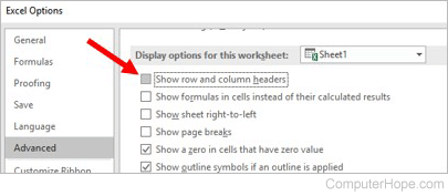
The column and row headers are now hidden. To display them again, re-check the box in step 4 above.
Format data as a table with header names
Formatting data in an Excel worksheet as a table helps make custom column headers in row 1 more prominent.
- Add custom column header names in row 1 using the steps above in the first section.
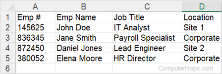
- Select all data in the worksheet, including row 1 with the header names.
- On the Home tab, click the Format as Table option in the Styles section.
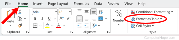
- Select the type of table to format the data. Table types with a background color in the first row help bring more attention to custom column header names.
- In the Create Table window, check the box for the My table has headers option, and then click OK.
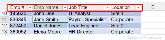
Additionally, when data is formatted as a table, select a cell in that table and scroll down in the worksheet. The default Excel column headers are replaced by the table's column headers.
Naming cells
If you want to change a row, column, or cell because it's hard to remember what cell contains what data, consider naming the cell to something easier to recall.
While cell naming is different than creating custom column headers, it helps identify data more clearly, similar to column header names.
For example, consider you have the value of each US state's tax rate in column M, but have difficulty remembering that Utah's state tax is in cell M46. Instead of referencing M46 in your Excel formulas, name the cell "UT" and use it in the formula. In other words, instead of using a formula like =SUM(B13*M56), it would be =SUM(B13*UT), which is easier to remember and reference. If this was done for every US state, calculations can be done a lot faster. See the following page for information about naming cells.