How to reference a cell from another cell in Microsoft Excel

When you are working with a spreadsheet in Microsoft Excel, it may be useful to create a formula that references the value of other cells. For instance, a cell's formula might calculate the sum of two other linked cells and display the result.
To accomplish this task, the formula must include at least one cell reference. In an Excel formula, a cell reference is used to reference the value of another cell.
Referencing a cell is useful to make automatic changes in one cell whenever data in another cell changes. For example, a financial spreadsheet might use cell references to add a budget for each week, and automatically calculate the budget for the entire year.
Cell references can access data on the same worksheet, or on other worksheets in the same workbook. For instructions on how to reference a cell, choose from the sections below.
Reference a cell in the current worksheet
If the cell you want to reference is in the same worksheet, follow the steps below to reference it.
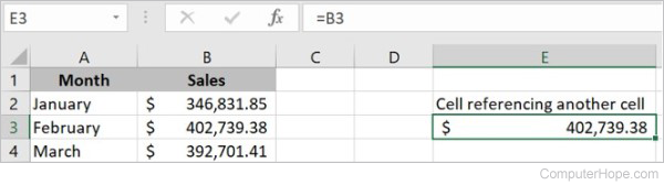
- Click the cell where you want to enter a reference to another cell.
- Type an equals (=) sign in the cell.
- Click the cell in the same worksheet you want to make a reference to, and the cell name is automatically entered after the equal sign. Press Enter to create the cell reference.
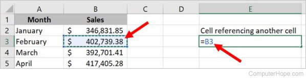
For example, we click the B3 cell, resulting in the cell containing the reference to display "=B3" and mirror any data changes made in B3.
Reference a cell from another worksheet in the current workbook
If the cell you want to reference is in another worksheet that's in your workbook (the same Excel file), follow the following steps.
- Click the cell where you want to enter a reference to another cell.
- Type an equals (=) sign in the cell.
- Click the worksheet tab at the bottom of the Excel program window where the cell you want to reference is located. The formula bar automatically enters the worksheet name after the equals sign. An exclamation point is also added to the end of the worksheet name in the formula bar.
- Click the cell whose value you want to reference, and the formula bar automatically contains the cell name, after the worksheet name and exclamation point. Press Enter to create the cell reference.
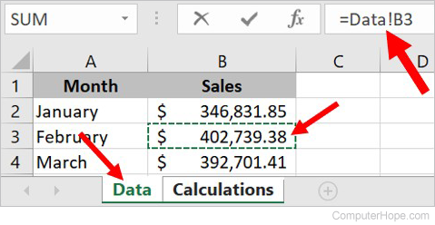
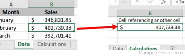
For example, we have a spreadsheet containing two worksheets named "Data" and "Calculations." In the Calculations worksheet, we want to reference a cell from the Data worksheet. We click the Data worksheet tab, then click the B3 cell, resulting in the formula bar displaying "=Data!B3" for the cell containing the reference. The data displayed in the Calculations worksheet mirrors the data in the B3 cell in the Data worksheet, and changes if the B3 cell changes.
Add two cells
You can perform mathematical operations on multiple cells by referencing them in a formula. For example, let's add two cells together, using the + (addition) operator in a formula.
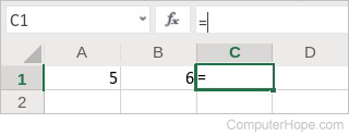
- In a new worksheet, enter two values in cells A1 and A2. In this example, we'll enter the value 5 in cell A1 and 6 in cell A2.
- Click cell C1 to select it. This cell contains our formula.
- Click inside the formula bar and type = to begin writing a formula.
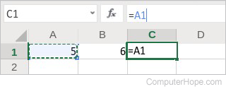
- Click cell A1 to automatically insert its cell reference in the formula.
- Type +.
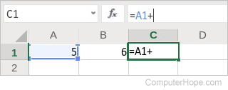
- Click cell B1 to automatically insert its cell reference in the formula.
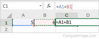
- Press Enter. Cell C1, containing your formula, automatically updates its value with the sum of 5 and 6.
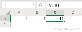
Now, if you change the values in cells A1 or B1, the value in C1 updates automatically.
You don't have to click the cells to insert their cell reference in the formula. If you prefer, with cell C1 selected, type =A1+B1 in the formula bar and press Enter.
Add up a range of cells
You can reference a range of cells in a formula by inserting a colon (:) between two cell references.
For example, you can add a range of values using the SUM() function. In this example, we show how you can sum an entire row or column of values, by specifying the range between two cell references.
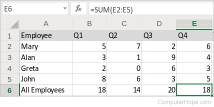
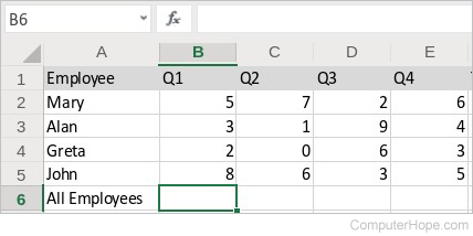
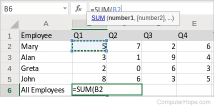
- Create a worksheet with multiple values that you want to sum up. In this example, we have a list of employees and how many sales they made each quarter. We want to find the quarterly totals for all employees combined.
- Let's create one sum. First, select the cell where you want the result displayed.
- Then, in the formula bar, type = to begin writing a formula. Then type the name of the function, SUM, and the open parenthesis (. Don't close the parentheses yet. Inside the parentheses, we're going to specify our range of cells to sum up.
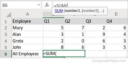
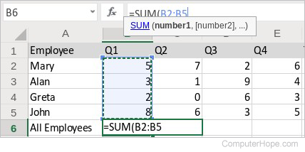
- Click the first value in the range. Here, we want to sum up the values in cells B2 through B5, so click the cell B2.
- Now, press and hold the Shift key, and click cell B5. By holding Shift, you're telling Excel that you want to add to your current selection, and include all the cells between. The cells are highlighted on your worksheet, and in the formula, the range B2:B5 is automatically inserted.
- Press Enter to complete the formula. Excel automatically inserts the closing parenthesis ) to complete the formula, and the result is displayed in the cell B6.
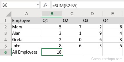
- You can repeat this process for each column to create sums for each quarter.