
How to create a pivot table in Microsoft Excel
A pivot table is a summary of a larger set of information stored in a spreadsheet or database. It's used as a way to quickly view totals, provide average values, or display data in a categorized method for review. In business, pivot tables are frequently used to provide an overview of sales data or business costs.
Microsoft Excel is a popular program for creating pivot tables. It works with small or large amounts of spreadsheet data to manipulate and organize data for review and to find trends and insights.
To create or edit a pivot table from your data, click the appropriate link below.
Create a pivot table
To create a pivot table in Microsoft Excel, follow the steps below.
- Open the Excel spreadsheet containing the data you want to use to create a pivot table.
- Create a new, blank worksheet in the spreadsheet. The new worksheet is where the pivot table is created.
- Click the new worksheet tab.
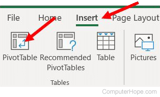
- In the Ribbon, click the Insert tab.
- On the Insert tab, click the Pivot Table option.
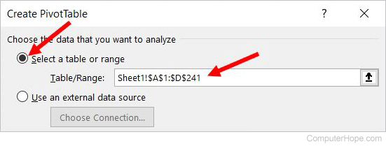
- The Create PivotTable window opens. The Select a table or range option is automatically selected. Click the worksheet containing the data for the pivot table and select all the cells with data. The Table/Range field on the Create PivotTable window is automatically populated with the worksheet name and selected range of cells.
- Click OK on the Create PivotTable window. The PivotTable Fields editor opens on the right side of the Excel program window.
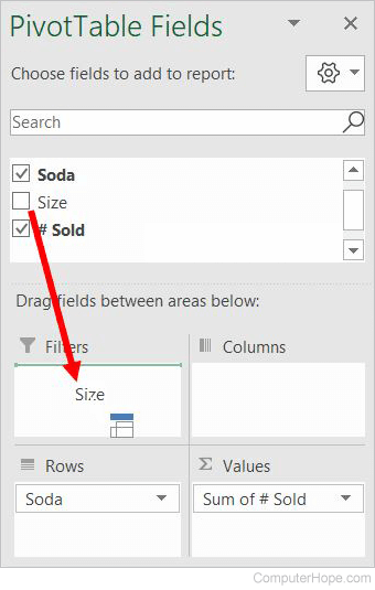
- The editor lists the fields (columns) from the selected range of cells. It also displays four options for how to display those fields of data: Columns, Filters, Rows, and Values. Drag-and-drop each column in the list to one of the four pivot table options.
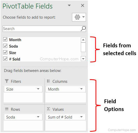
The Columns and Filters options are optional and are not required for creating a pivot table.
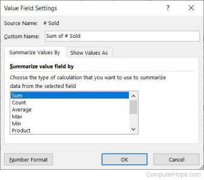
For any field added to the Values option, you can change the settings for the field to Sum, Count, Average, Min, Max, and more. To do so, click the down arrow next to the field name, select Value Field Settings in the drop-down menu, select the desired setting, and click OK.
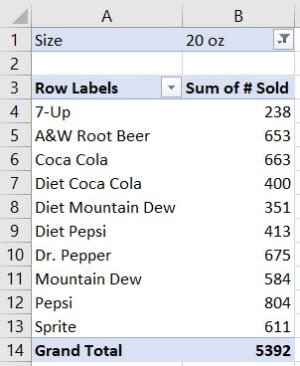
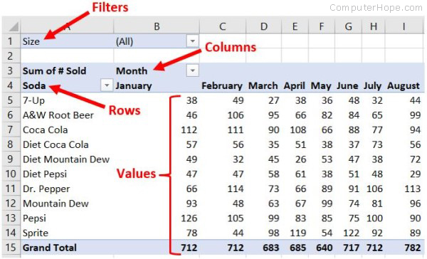
- As you add fields to each pivot table option in the editor, the pivot table is created in the worksheet. Below is an example of a pivot table, based on the pivot table editor screenshot above.
Edit a pivot table
To edit a pivot table in Microsoft Excel, follow the steps below.
- Open the Excel spreadsheet with the pivot table.
- Click anywhere in the pivot table. The PivotTable Fields section opens on the right side of the Excel program window.
- Add or remove fields to any of the four options (Columns, Fields, Rows, Values) by dragging and dropping a field to or from the option boxes.
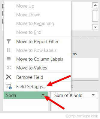
- To change a fields settings in any of the four options, click the down arrow next to the field name and select Field Settings.
- In the Field Settings window, make the desired changes to the settings and click OK.
- You can also edit the font type, size, color, and style (bold, italics, underlined, etc.) for text and data in any cell of the pivot table. Click a cell and make the desired text formatting changes.