Conditional formatting

Conditional formatting is a feature included in the popular spreadsheet creation programs Excel and Google Sheets. This feature automatically applies formatting, such as font color or bolding, to a cell when the data in that cell meets specific criteria. For example, in the image, the font color is automatically changed to red in all cells with negative values.

Using conditional formatting in Excel

To add conditional formatting to an Excel workbook, follow the steps below.

1. Open or create an Excel workbook.
2. Select the desired range of cells. You may also select the entire workbook using Ctrl+A.
3. On the Home tab, select the Conditional Formatting option, then select New Rule.
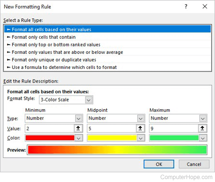
4. In the New Formatting Rule window, select the type of rule you want to create under Select a Rule Type.
5. Under Edit the Rule Description, select the desired Format Style, and select or enter the necessary criteria for the Rule Type and Format Style selected.
6. Click OK to save and apply the rule to the selected cells.

Using conditional formatting in Google Sheets

To add conditional formatting to a Google Sheets workbook, follow the steps below.

1. Go to the Google Sheets website and open or create a workbook.
2. Select the desired range of cells. You may also select the entire workbook using Ctrl+A.
3. Select Format from the menu bar and click Conditional Formatting.
4. For a rule with only one format, select the Single color tab. For a rule that affects different values differently, select Color scale.
5. Under Format rules, select the rules you want the selected text to follow.
6. Under Formatting style, select how the affected text is displayed.
7. Select the Done button to add the rule.

Bolding, Cell, Google, Microsoft, Software terms, Spreadsheet